Normal random variables
If the probability density of a continuous random variable $ X $ has the following form, then the random variable is called normal or Gaussian.
$$
f_X(x)=\frac{1}{\sqrt{2\pi}\sigma}e^{\frac{-(x-\mu)^2}{2\sigma^2}}
$$
Among them, $ u $ and $ \ sigma $ are two parameters of the density function, and $ \ sigma $ must also be a positive number. It can be proved that $ f_X (x) $ satisfies the normalization condition of the following probability density function (see the exercises on theorems in this chapter):
$$
\frac{1}{\sqrt{2\pi}\sigma}\int_{-\infty}^{+\infty}e^{\frac{-(x-\mu)^2}{2\sigma^2}}dx=1
$$
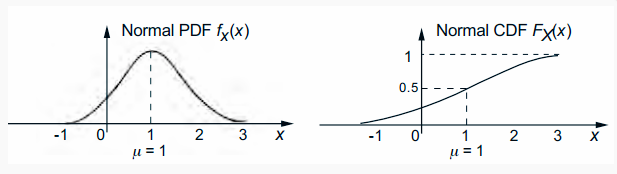
The figure below is the density function and distribution function of the normal distribution $ (\mu=1 \text{ and } \sigma^2=1) $.
 [Figure : [A_normal_PDF_and_CDF_with_u = 1_and_sigmal ^ 2 = 1]
It can be seen from the figure that the probability density function of a normal random variable is a symmetrical bell curve with respect to the mean $ \ mu $. When $ x $ leaves $ \ mu $, the term $ e ^ {\ frac {-(x- \ mu) ^ 2} {2 \ sigma ^ 2}} $ in the expression of the probability density function quickly decline. In the figure, the probability density function is very close to $ 0 $ outside the interval $ [-1,3] $.
The mean and variance of a normal random variable can be given by the following formula:
$$
E[X]=\mu,\quad var(X)=\sigma^2
$$
Since the probability density function of $ X $ is symmetric with respect to $ \ mu $, its mean can only be $ \ mu $. As for the formula of variance, one sentence is defined as:
$$
var(X)=\frac{1}{\sqrt{2\pi}\sigma}\int_{-\infty}^{+\infty}(x-\mu)^2e^{-\frac{(x-\mu)^2}{2\sigma^2}}dx
$$
Replacing the integral in the formula as an integral variable $ y = \ frac { ( x - \ mu ) } { \ sigma } $ and the distributed integral yields:
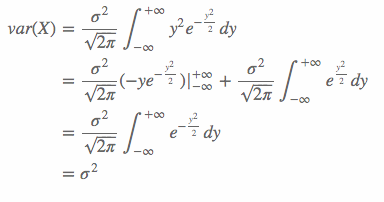
The last equation above is due to
$$
\frac{1}{\sqrt{2\pi}}\int_{-\infty}^{+\infty}e^{-\frac{y^2}{2}}dy=1
$$
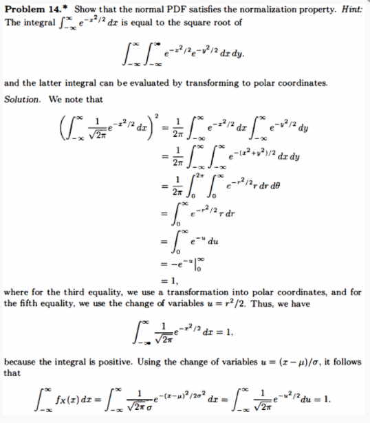
This formula happens to be the normalization condition of the probability density function of the normal random variable when $ \ mu = 0 $ and $ \ sigma ^ 2 = 1 $. The problem is proved in the problem 14 of this chapter. The screenshot is as follows:
 [Figure : the_normal_PDF_satisfies_the_normalization_property]
Normal random variables have several important properties. The following properties are particularly important and will be discussed in Chapter 4 This is demonstrated in the first section of on Random Variables.
The normality of random variables remains unchanged under linear transformation
Let $ X $ be a normal random variable, the mean of which is $ \ mu $ and the variance is $ \ sigma ^ 2 $. If $ a \ ne 0 $ and $ b $ are two constants, then the random variable
$$
Y = aX + b
$$
It is still a normal random variable, and its mean and variance are given by the following formula:
$$
E[Y]=a\mu+b,\quad var(Y)=a^2\sigma^2
$$
Standard normal random variables
Suppose the expectation of the normal random variable $ Y $ is $ 0 $ and the variance is $ 1 $, then $ Y $ is called the standard normal random variable. Let $ \ Phi $ be its CDF:
$$
\Phi(y)=P(Y\le y)=P(Y< y)=\frac{1}{\sqrt{2\pi}}\int_{-\infty}^{y}e^{\frac{-t^2}{2}}dt
$$
It is usually listed as a table-the standard normal cumulative distribution table (see the table below), which is an important tool for calculating the probability of normal random variables. Each item of the standard normal table provides the value of $ \Phi(y)=P(Y\le y) $, where $ Y $ is a normal random variable, and in this table $ y\in [0,4.09] $. How to use this table? For example, to find the value of $ \Phi(1.71) $, look at the row where $ 1.7 $ is located and the column where $ 0.01 $ is located, and you get $ \Phi(1.71)=0.95637 $.
Note that the following table only lists the value of $ \Phi ( y ) $ when y> 0, the symmetry of the probability density function of the standard normal random variable can be used, and $ \Phi ( y ) $ The value is derived. E.g:
= 1− Φ (0.5) = 1 − 0.69146 = 0.30854
∀ y> 0 , Φ(−y)= 1 − Φ (y)
| y | +0.00 | +0.01 | +0.02 | +0.03 | +0.04 | +0.05 | +0.06 | +0.07 | +0.08 | +0.09 |
|---|---|---|---|---|---|---|---|---|---|---|
| 0.0 | 0.50000 | 0.50399 | 0.50798 | 0.51197 | 0.51595 | 0.51994 | 0.52392 | 0.52790 | 0.53188 | 0.53586 |
| 0.1 | 0.53983 | 0.54380 | 0.54776 | 0.55172 | 0.55567 | 0.55966 | 0.56360 | 0.56749 | 0.57142 | |
| 0.2 | 0.57926 | 0.58317 | 0.58706 | 0.59095 | 0.59483 | 0.59871 | 0.60257 | 0.60642 | 0.61026 | |
| 0.3 | 0.61791 | 0.62172 | 0.62552 | 0.62930 | 0.63307 | 0.63683 | 0.64058 | 0.64431 | 0.64803 | 0.65173 |
| 0.4 | 0.65542 | 0.65910 | 0.66276 | 0.66640 | 0.67003 | 0.67364 | 0.67724 | 0.68082 | 0.68439 | |
| 0.5 | 0.69146 | 0.69497 | 0.69847 | 0.70194 | 0.70540 | 0.70884 | 0.71226 | 0.71566 | 0.71904 | 0.72240 |
| 0.6 | 0.72575 | 0.72907 | 0.73237 | 0.73565 | 0.73891 | 0.74215 | 0.74537 | 0.74857 | 0.75175 | |
| 0.7 | 0.75804 | 0.76115 | 0.76424 | 0.76730 | 0.77035 | 0.77337 | 0.77637 | 0.77935 | 0.78230 | 0.78524 |
| 0.8 | 0.78814 | 0.79103 | 0.79389 | 0.79673 | 0.79955 | 0.80234 | 0.80511 | 0.80785 | 0.81057 | 0.81327 |
| 0.9 | 0.81594 | 0.81859 | 0.82121 | 0.82381 | 0.82639 | 0.82894 | 0.83147 | 0.83398 | 0.83646 | 0.83891 |
| 1.0 | 0.84134 | 0.84375 | 0.84614 | 0.84849 | 0.85083 | 0.85314 | 0.85543 | 0.85769 | 0.85993 | |
| 1.1 | 0.86433 | 0.86650 | 0.86864 | 0.87076 | 0.87286 | 0.87493 | 0.87698 | 0.87900 | 0.88100 | |
| 1.2 | 0.88493 | 0.88686 | 0.88877 | 0.89065 | 0.89251 | 0.89435 | 0.89617 | 0.89796 | 0.89973 | |
| 1.3 | 0.90320 | 0.90490 | 0.90658 | 0.90824 | 0.90988 | 0.91149 | 0.91308 | 0.91466 | 0.91621 | 0.91774 |
| 1.4 | 0.91924 | 0.92073 | 0.92220 | 0.92364 | 0.92507 | 0.92647 | 0.92785 | 0.92922 | 0.93056 | 0.93189 |
| 1.5 | 0.93319 | 0.93448 | 0.93574 | 0.93699 | 0.93822 | 0.93943 | 0.94062 | 0.94179 | 0.94295 | 0.94408 |
| 1.6 | 0.94520 | 0.94630 | 0.94738 | 0.94845 | 0.94950 | 0.95053 | 0.95154 | 0.95254 | 0.95352 | 0.95449 |
| 1.7 | 0.95543 | 0.95637 | 0.95728 | 0.95818 | 0.95907 | 0.95994 | 0.96080 | 0.96164 | 0.96246 | 0.96327 |
| 1.8 | 0.96407 | 0.96485 | 0.96562 | 0.96638 | 0.96712 | 0.96784 | 0.96856 | 0.96926 | 0.96995 | 0.97062 |
| 0.99128 | 0.97193 | 0.97257 | 0.97320 | 0.97381 | 0.97441 | 0.97500 | 0.97558 | 0.97615 | 0.97670 | |
| 2.0 | 0.97725 | 0.97778 | 0.97831 | 0.97882 | 0.97932 | 0.97982 | 0.98030 | 0.98077 | 0.98124 | 0.98169 |
| 2.1 | 0.98214 | 0.98257 | 0.98300 | 0.98341 | 0.98382 | 0.98422 | 0.98461 | 0.98500 | 0.98537 | |
| 2.2 | 0.98610 | 0.98645 | 0.98679 | 0.98713 | 0.98745 | 0.98778 | 0.98809 | 0.98840 | 0.98870 | |
| 2.3 | 0.98928 | 0.98956 | 0.98983 | 0.99010 | 0.99036 | 0.99061 | 0.99086 | 0.99111 | 0.99134 | 0.99158 |
| 2.4 | 0.99180 | 0.99202 | 0.99224 | 0.99245 | 0.99266 | 0.99286 | 0.99305 | 0.99324 | 0.99343 | 0.99361 |
| 2.5 | 0.99379 | 0.99396 | 0.99413 | 0.99430 | 0.99446 | 0.99461 | 0.99477 | 0.99492 | 0.99506 | 0.99520 |
| 2.6 | 0.99534 | 0.99547 | 0.99560 | 0.99573 | 0.99585 | 0.99598 | 0.99609 | 0.99621 | 0.99632 | 0.99643 |
| 2.7 | 0.99653 | 0.99664 | 0.99674 | 0.99683 | 0.99693 | 0.99702 | 0.99711 | 0.99720 | 0.99728 | 0.99736 |
| 2.8 | 0.99744 | 0.99752 | 0.99760 | 0.99767 | 0.99774 | 0.99781 | 0.99788 | 0.99795 | 0.99801 | 0.99807 |
| 2.9 | 0.99813 | 0.99819 | 0.99825 | 0.99831 | 0.99836 | 0.99841 | 0.99846 | 0.99851 | 0.99856 | 0.99861 |
| 3.0 | 0.99865 | 0.99869 | 0.99874 | 0.99878 | 0.99882 | 0.99886 | 0.99889 | 0.99893 | 0.99896 | 0.99900 |
| 3.1 | 0.99903 | 0.99906 | 0.99910 | 0.99913 | 0.99916 | 0.99918 | 0.99921 | 0.99924 | 0.99926 | 0.99929 |
| 3.2 | 0.99931 | 0.99934 | 0.99936 | 0.99938 | 0.99940 | 0.99942 | 0.99944 | 0.99946 | 0.99948 | 0.99950 |
| 3.3 | 0.99952 | 0.99953 | 0.99955 | 0.99957 | 0.99958 | 0.99960 | 0.99961 | 0.99962 | 0.99964 | 0.99965 |
| 3.4 | 0.99966 | 0.99968 | 0.99969 | 0.99970 | 0.99971 | 0.99972 | 0.99973 | 0.99974 | 0.99975 | 0.99976 |
| 3.5 | 0.99977 | 0.99978 | 0.99978 | 0.99979 | 0.99980 | 0.99981 | 0.99981 | 0.99982 | 0.99983 | 0.99983 |
| 3.6 | 0.99984 | 0.99985 | 0.99985 | 0.99986 | 0.99986 | 0.99987 | 0.99987 | 0.99988 | 0.99988 | 0.99989 |
| 3.7 | 0.99989 | 0.99990 | 0.99990 | 0.99990 | 0.99991 | 0.99991 | 0.99992 | 0.99992 | 0.99992 | 0.99992 |
| 3.8 | 0.99993 | 0.99993 | 0.99993 | 0.99994 | 0.99994 | 0.99994 | 0.99994 | 0.99995 | 0.99995 | 0.99995 |
| 3.9 | 0.99995 | 0.99995 | 0.99996 | 0.99996 | 0.99996 | 0.99996 | 0.99996 | 0.99996 | 0.99997 | 0.99997 |
| 4.0 | 0.99997 | 0.99997 | 0.99997 | 0.99997 | 0.99997 | 0.99997 | 0.99998 | 0.99998 | 0.99998 | 0.99998 |
Now use $ X $ to represent a normal random variable with a mean of $ \ mu $ and a variance of $ \ sigma ^ 2 $. Standardize $ X $ (“standardize”) by defining a new random variable $ Y $:
$$
Y=\frac{X-\mu}{\sigma}
$$
Because $ Y $ is a linear function of $ X $, $ Y $ is also a normal random variable. and
$$
E[Y]=\frac{E[X]-u}{\sigma}=0,\quad var(Y)=\frac{var(X)}{\sigma^2}=1
$$
Therefore, $ Y $ is a standard normal random variable. This fact allows us to redefine the event represented by $ X $ with $ Y $, and then use the standard normal table to calculate.
Example of using normal distribution table
The annual snowfall in a certain area is a normal random variable, the expectation is $ \ mu = 60 $ inches, and the standard deviation is $ \ sigma = 20 $. What is the probability that the snowfall will be at least $ 80 $ inches this year?
Let $ X $ be the annual snowfall, so that
$$
Y=\frac{X-\mu}{\sigma}=\frac{X-60}{20}
$$
Obviously $ Y $ is a standard normal random variable.
$$
P(X\ge 80)=P(\frac{X-60}{20} \ge \frac{80-60}{20})=P(Y\ge \frac{80-60}{20})=P(Y\ge 1)=1-\Phi(1)
$$
Where $ \ Phi $ is the standard normal cumulative distribution function. Obtained by querying the above table: $ \Phi(1)=0.84134 $, so
$$
P(X\ge 80)=1-\Phi(1)=0.15866
$$
Promoting the method in this example, we get the following:
Calculation of the cumulative distribution function of normal random variables
For a normal random variable $ X $ with a mean of $ \ mu $ and a variance of $ \ sigma ^ 2 $, use the following steps:
Normalized $ X $: First subtract $ \ mu $ and then divide by $ \ sigma $ to obtain the standard random variable $ Y $.
Read the cumulative distribution function value from the standard normal table:
$$
P(X\le x)=P(\frac{X-\mu}{\sigma}\le \frac{x-\mu}{\sigma})=P(Y\le \frac{x-\mu}{\sigma})=\Phi(\frac{x-\mu}{\sigma})
$$
Normal random variables are often used in signal processing and communication engineering to model noise and signal distortion.
Example 3.8 Signal detection
Binary information is transmitted with the signal $ s $. This information is either $ -1 $ and $ + 1 $. The signal will be accompanied by some noise during the channel transmission. The noise satisfies the normal distribution with a mean value of $ \ mu = 0 $ and a variance of $ \ sigma ^ 2 $. The receiver will receive a signal mixed with noise, if the received value is less than $ 0 $, then the signal is considered to be $ -1 $, if the received value is greater than $ 0 $, then the received signal is considered to be $ + 1 $. How big is the error of this judgment method?
The error only appears in the following two cases:
- The actual transmitted signal is $ -1 $, but the value of the noise variable $ N $ is at least $ 1 $, so $ s + N = -1 + N \ ge 0 $.
- The actual transmitted signal is $ + 1 $, but the value of the noise variable $ N $ is less than $ -1 $. Therefore $ s + N = 1 + N <0 $.
[Figure_3.11_The_signal_detection]
Therefore, the probability of error in this judgment method in case 1 is:
P ( N ≥ 1 ) = 1 − P ( N < 1 ) = 1 − P ( N < 1 ) = 1 − P ( N − Μ / σ < 1 − μ ) / σ )
= 1 - Φ( 1 − μ ) / σ)
= 1 - Φ( 1 / σ)
The probability of an error in the second case is obtained according to the symmetry of the normal distribution as in the previous case. $ \Phi (\frac {1} {\sigma}) $ can be obtained from the normal distribution table. For example, for $ \sigma = 1 $, $ \Phi (\frac {1} {\ sigma}) = \Phi (1) = 0.84134 $, so the probability of error is $ 0.15864 $.
Normal random variables play an important role in a wide range of probabilistic models. The reason is that normal random variables can well simulate the superposition effect of many independent factors in physics, engineering and statistics. Mathematically, the key fact is that the distribution of the sum of a large number of independent and identically distributed random variables (not necessarily normal) obey the normal distribution, and this fact has nothing to do with the specific distribution of each sum.