Note - These are my notes on DeepLearning Specialization Part:
Regularization || Deeplearning (Course - 2 Week - 1) || Improving Deep Neural Networks(Week 1)
Introduction:
If you suspect your neural network is over fitting your data. That is you have a high variance problem, one of the first things you should try per probably regularization. The other way to address high variance, is to get more training data that's also quite reliable. But you can't always get more training data, or it could be expensive to get more data. But adding regularization will often help to prevent overfitting, or to reduce the errors in your network. So let's see how regularization works. Let's develop these ideas using logistic regression. Recall that for logistic regression, you try to minimize the cost function J, which is defined as this cost function. In other words, instead of simply aiming to minimize loss (empirical risk minimization): Because here, you're using the Euclidean normals, or else the L2 norm with the prime to vector w. Now, why do you regularize just the parameter w? Why don't we add something here about b as well? In practice, you could do this, but I usually just omit this. Because if you look at your parameters, w is usually a pretty high dimensional parameter vector, especially with a high variance problem. Maybe w just has a lot of parameters, so you aren't fitting all the parameters well, whereas b is just a single number. So almost all the parameters are in w rather b. And if you add this last term, in practice, it won't make much of a difference, because b is just one parameter over a very large number of parameters. In practice, I usually just don't bother to include it. But you can if you want. So L2 regularization is the most common type of regularization. You might have also heard of some people talk about L1 regularization. And that's when you add, instead of this L2 norm, you instead add a term that is lambda/m of sum over of this. And this is also called the L1 norm of the parameter vector w, so the little subscript 1 down there, right? And I guess whether you put m or 2m in the denominator, is just a scaling constant. L1 Regularization If you use L1 regularization, then w will end up being sparse. And what that means is that the w vector will have a lot of zeros in it. And some people say that this can help with compressing the model, because the set of parameters are zero, and you need less memory to store the model. Although, I find that, in practice, L1 regularization to make your model sparse, helps only a little bit. So I don't think it's used that much, at least not for the purpose of compressing your model. And when people train your networks, L2 regularization is just used much much more often. Sorry, just fixing up some of the notation here. So one last detail. Lambda here is called the regularization, Parameter.And usually, you set this using your development set, or using [INAUDIBLE] cross validation. When you a variety of values and see what does the best, in terms of trading off between doing well in your training set versus also setting that two normal of your parameters to be small. Which helps prevent over fitting. So lambda is another hyper parameter that you might have to tune. And by the way, for the programming exercises, lambda is a reserved keyword in the Python programming language. So in the programming exercise, we’ll have lambd,
]without the a, so as not to clash with the reserved keyword in Python. So we use lambd to represent the lambda regularization parameter.
$$
\text{minimize(Loss(Data|Model))}
$$
we’ll now minimize loss+complexity, which is called structural risk minimization:
$$\text{minimize(Loss(Data|Model) + complexity(Model))}$$
Our training optimization algorithm is now a function of two terms: the loss term, which measures how well the model fits the data, and the regularization term, which measures model complexity.
Model complexity as a function of the weights of all the features in the model.
Model complexity as a function of the total number of features with nonzero weights. (A later module covers this approach.)
If model complexity is a function of weights, a feature weight with a high absolute value is more complex than a feature weight with a low absolute value.
We can quantify complexity using the L2 regularization formula, which defines the regularization term as the sum of the squares of all the feature weights:
$$
L_2 \text{ regularization term} = ||\boldsymbol w||_2^2 = {w_1^2 + w_2^2 + … + w_n^2}
$$
In this formula, weights close to zero have little effect on model complexity, while outlier weights can have a huge impact.
For example, a linear model with the following weights:
$$
{w_1 = 0.2, w_2 = 0.5, w_3 = 5, w_4 = 1, w_5 = 0.25, w_6 = 0.75}
$$
Has an L2 regularization term of 26.915:
$$
w_1^2 + w_2^2 + \boldsymbol{w_3^2} + w_4^2 + w_5^2 + w_6^2$$ $$= 0.2^2 + 0.5^2 + \boldsymbol{5^2} + 1^2 + 0.25^2 + 0.75^2$$ $$= 0.04 + 0.25 + \boldsymbol{25} + 1 + 0.0625 + 0.5625
$$
$$
= 26.915$$
But (w_3) (bolded above), with a squared value of 25, contributes nearly all the complexity. The sum of the squares of all five other weights adds just 1.915 to the L2 regularization term.
Lambda Introduction
Model developers tune the overall impact of the regularization term by multiplying its value by a scalar known as lambda (also called the regularization rate). That is, model developers aim to do the following:$$ \text{minimize(Loss(Data|Model)} + \lambda \text{ complexity(Model))} $$
Performing L2 regularization has the following effect on a model
Encourages weight values toward 0 (but not exactly 0)
Encourages the mean of the weights toward 0, with a normal (bell-shaped or Gaussian) distribution.
Increasing the lambda value strengthens the regularization effect. For example, the histogram of weights for a high value of lambda
Some of your training examples of the losses of the individual predictions in the different examples, where you recall that w and b in the logistic regression, are the parameters. So w is an x-dimensional parameter vector, and b is a real number. And so to add regularization to the logistic regression, what you do is add to it this thing, lambda, which is called the regularization parameter. I’ll say more about that in a second. But lambda/2m times the norm of w squared. So here, the norm of w squared is just equal to sum from j equals 1 to nx of wj squared, or this can also be written w transpose w, it’s just a square Euclidean norm of the prime to vector w. And this is called L2 regularization.
When choosing a lambda value, the goal is to strike the right balance between simplicity and training-data fit:
If your lambda value is too high, your model will be simple, but you run the risk of underfitting your data. Your model won’t learn enough about the training data to make useful predictions.
If your lambda value is too low, your model will be more complex, and you run the risk of overfitting your data. Your model will learn too much about the particularities of the training data, and won’t be able to generalize to new data.
Note: Setting lambda to zero removes regularization completely. In this case, training focuses exclusively on minimizing loss, which poses the highest possible overfitting risk.
The ideal value of lambda produces a model that generalizes well to new, previously unseen data. Unfortunately, that ideal value of lambda is data-dependent, so you’ll need to do some tuning.
L2 Regularization and lambda (Regularization Parameter): relation
There’s a close connection between learning rate and lambda. Strong L2 regularization values tend to drive feature weights closer to 0. Lower learning rates (with early stopping) often produce the same effect because the steps away from 0 aren’t as large. Consequently, tweaking learning rate and lambda simultaneously may have confounding effects.
Early stopping means ending training before the model fully reaches convergence. In practice, we often end up with some amount of implicit early stopping when training in an online (continuous) fashion. That is, some new trends just haven’t had enough data yet to converge.
As noted, the effects from changes to regularization parameters can be confounded with the effects from changes in learning rate or number of iterations. One useful practice (when training across a fixed batch of data) is to give yourself a high enough number of iterations that early stopping doesn’t play into things.
Implementing L2 Regularisation in a Neural Network
So this is how you implement L2 regularization for logistic regression. How about a neural network? In a neural network, you have a cost function(J) that's a function of all of your parameters, w[1], b[1] through w[L], b[L], where capital L is the number of layers in your neural network. And so the cost function is this, sum of the losses, summed over your m training examples.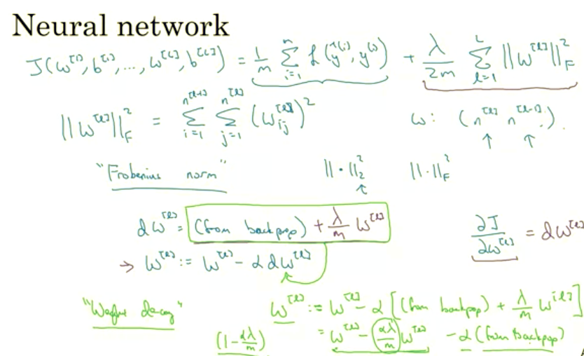
L2 Norm ~ Weight Deacy
And it's for this reason that L2 regularization is sometimes also called weight decay. So if I take this definition of dw[l] and just plug it in here, then you see that the update is w[l] = w[l] times the learning rate alpha times the thing from backprop, +lambda of m times w[l]. Throw the minus sign there. And so this is equal to $$ (w[l]- alpha * lambda / m) * (w[l]- alpha) $$ times the thing you got from backpop. And so this term shows that whatever the matrix w[l] is, you're going to make it a little bit smaller, right? This is actually as if you're taking the matrix w and you're multiplying it by $$ 1-alpha*lambda/m$$ . You're really taking the matrix w and subtracting $$ alpha*lambda/m $$ with L2 Regularization penalty . Like you're multiplying matrix w by this number, which is going to be a little bit less than 1. So this is why L2 norm regularization is also called weight decay. Because it's just like the ordinally gradient descent, where you update w by subtracting alpha times the original gradient you got from backprop. But now you're also multiplying w by this thing, which is a little bit less than 1. So the alternative name for L2 regularization is weight decay. I'm not really going to use that name, but the intuition for it's called weight decay is that this first term here, is equal to this. So you're just multiplying the weight metrics by a number slightly less than 1. So that's how you implement L2 regularization in neural network. Now, one question that he has asked me is, why does regularization prevent over-fitting? Let's look at the next Section, and gain some intuition for how regularization prevents over-fitting.How do regularization Prevent Overfitting?
Why does regularization help with overfitting? Why does it help with reducing variance problems? Let's go through a couple examples to gain some intuition about how it works. So, recall that high bias, high variance. And I just write pictures from our earlier section that looks something like this.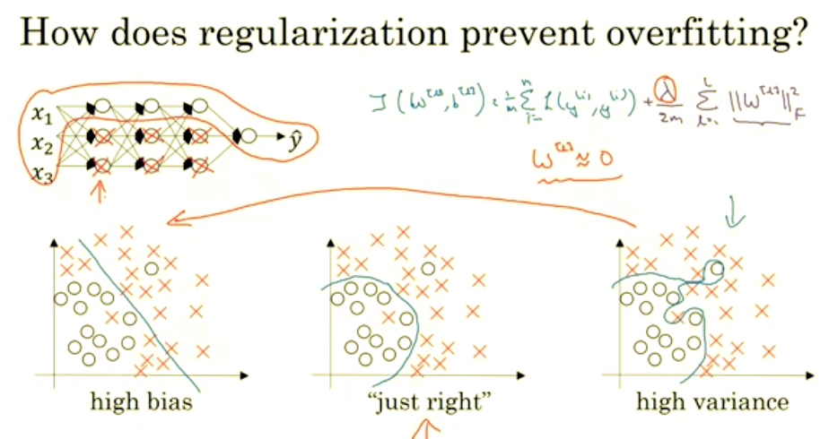
$$\text{minimize(Loss(Data|Model)} + \lambda \text{ complexity(Model))}$$
So what we did for regularization was add this extra term that penalizes the weight matrices from being too large. So that was the Frobenius norm. So why is it that shrinking the L two norm or the Frobenius norm or the parameters might cause less overfitting? One piece of intuition is that if you crank regularisation lambda to be really, really big, they’ll be really incentivized to set the weight matrices W to be reasonably close to zero. So one piece of intuition is maybe it set the weight to be so close to zero for a lot of hidden units that’s basically zeroing out a lot of the impact of these hidden units. And if that’s the case, then this much simplified neural network becomes a much smaller neural network. In fact, it is almost like a logistic regression unit, but stacked most probably as deep. And so that will take you from this overfitting case much closer to the left to other high bias case. But hopefully there’ll be an intermediate value of lambda that results in a result closer to this just right case in the middle.
But the intuition is that by cranking up lambda to be really big they’ll set W close to zero, which in practice this isn’t actually what happens. We can think of it as zeroing out or at least reducing the impact of a lot of the hidden units so you end up with what might feel like a simpler network.
They get closer and closer as if you’re just using logistic regression.
The intuition of completely zeroing out of a bunch of hidden units isn’t quite right.
It turns out that what actually happens is they’ll still use all the hidden units, but each of them would just have a much smaller effect. But you do end up with a simpler network and as if you have a smaller network that is therefore less prone to overfitting.
So a lot of this intuition helps better when you implement regularization in the program exercise, you actually see some of these variance reduction results yourself.
Another Intution with TanH as activation Function instead of Sigmoid
Here's another attempt at additional intuition for why regularization helps prevent overfitting. And for this, I'm going to assume that we're using the tanh activation function which looks like this.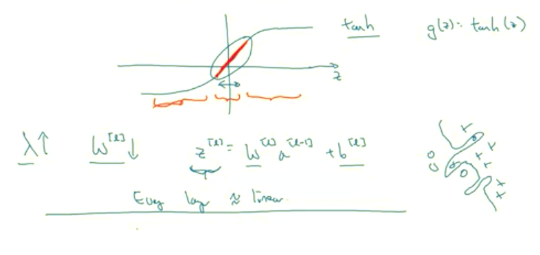
Takeaway:
So the intuition you might take away from this is that if lambda, the regularization parameter, is large, then you have that your parameters will be relatively small, because they are penalized being large into a cos function. And so if the blades W are small then because Z is equal to W and then technically is plus b, but if W tends to be very small, then Z will also be relatively small. And in particular, if Z ends up taking relatively small values, just in this whole range, then G of Z will be roughly linear. So it's as if every layer will be roughly linear. As if it is just linear regression. And we saw in course one that if every layer is linear then your whole network is just a linear network. And so even a very deep network, with a deep network with a linear activation function is at the end they are only able to compute a linear function. So it's not able to fit those very very complicated decision. Very non-linear decision boundaries that allow it to really overfit right to data sets like we saw on the overfitting high variance case on the previous slide.So just to summarize
If the regularization becomes very large, the parameters W very small, so Z will be relatively small, kind of ignoring the effects of b for now, so Z will be relatively small or, really,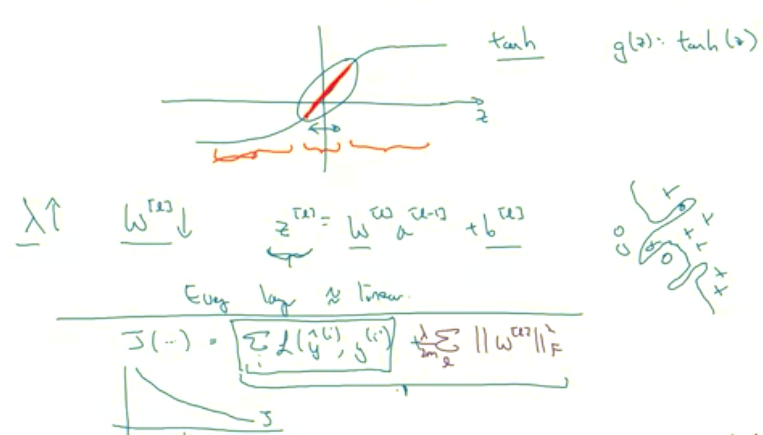
Tip
Before wrapping up our def discussion on regularization, I just want to give you one implementational tip. Which is that, when implanting regularization, we took our definition of the cost function J and we actually modified it by adding this extra term that penalizes the weight being too large. And so if you implement gradient descent, one of the steps to debug gradient descent is to plot the cost function J as a function of the number of elevations of gradient descent and you want to see that the cost function J decreases monotonically after every elevation of gradient descent. And if you're implementing regularization then please remember that J now has this new definition. If you plot the old definition of J, just this first term, then you might not see a decrease monotonically. So to debug gradient descent make sure that you're plotting this new definition of J that includes this second term as well. Otherwise you might not see J decrease monotonically on every single elevation. So that's it for L two regularization which is actually a regularization technique that I use the most in training deep learning modules. In deep learning there is another sometimes used regularization technique called dropout regularization. Let's take a look at that in the next section.Dropout Regularization
In addition to L2 regularization, another very powerful regularization techniques is called "dropout." Let's see how that works. Let's say you train a neural network like the one on the left and there's over-fitting. Here's what you do with dropout. Let me make a copy of the neural network.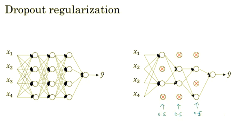
Implementing Dropout
Let's look at how you implement dropout. There are a few ways of implementing dropout. I'm going to show you the most common one, which is technique called inverted dropout. For the sake of completeness, let's say we want to illustrate this with layer l=3. So, in the code I'm going to write- there will be a bunch of 3s here. I'm just illustrating how to represent dropout in a single layer. So, what we are going to do is set a vector d and d^3 is going to be the dropout vector for the layer 3.Inverted Dropout
That's what the 3 is to be np.random.rand(a). And this is going to be the same shape as a3. And when I see if this is less than some number, which I'm going to call keep.prob. And so, keep.prob is a number. It was 0.5 on the previous time, and maybe now I'll use 0.8 in this example,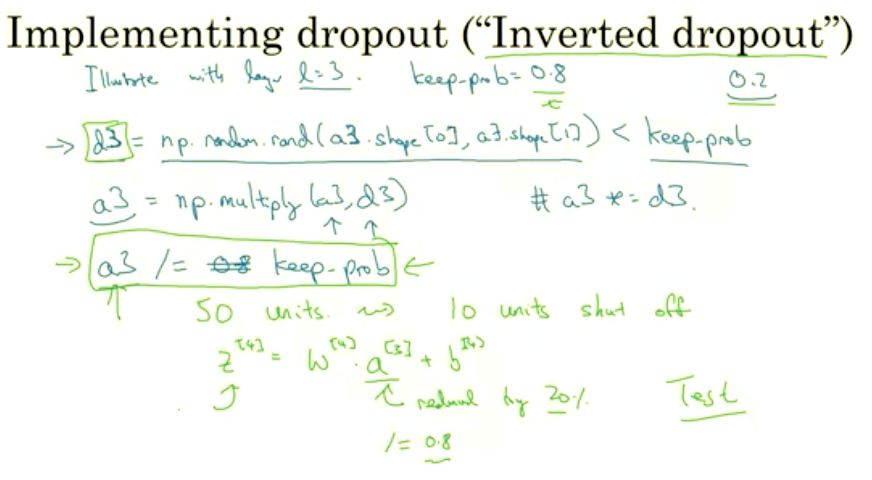
Introspect Results:
In theory, one thing you could do is run a prediction process many times with different hidden units randomly dropped out and have it across them. But that's computationally inefficient and will give you roughly the same result; very, very similar results to this different procedure as well. And just to mention, the inverted dropout thing, you remember the step on the previous line when we divided by the cheap.prob. The effect of that was to ensure that even when you don't see men dropout at test time to the scaling, the expected value of these activations don't change. So, you don't need to add in an extra funny scaling parameter at test time. That's different than when you have that training time. So that's dropouts. And when you implement this in week's premier exercise, you gain more firsthand experience with it as well. But why does it really work? What I want to do the next section is give you some better intuition about what dropout really is doing. Let's go on to the next section.Understanding Dropout
Drop out does this seemingly crazy thing of randomly knocking out units on your network. Why does it work so well with a regularizer? Let's gain some better intuition. In the previous section, I gave this intuition that drop-out randomly knocks out units in your network. So it's as if on every iteration you're working with a smaller neural network, and so using a smaller neural network seems like it should have a regularizing effect.Why Does Dropout Work ?
Here's a second intuition which is, let's look at it from the perspective of a single unit. Let's say this one. Now, for this unit to do his job as for inputs and it needs to generate some meaningful output. Now with drop out, the inputs can get randomly eliminated. Sometimes those two units will get eliminated, sometimes a different unit will get eliminated.
For clarity
These numbers I'm drawing on the purple boxes, These could be different key props for different layers. Notice that the key prop of one point zero means that you're keeping every unit and so, you're really not using drop out for that layer. But for layers where you're more worried about over-fitting, really the layers with a lot of parameters, you can set the key prop to be smaller to apply a more powerful form of drop out. It's kind of like cranking up the regularization parameter lambda of L2 regularization where you try to regularize some layers more than others. And technically, you can also apply drop out to the input layer, where you can have some chance of just maxing out one or more of the input features. Although in practice, usually don't do that that often. And so, a key prop of one point zero was quite common for the input there. You can also use a very high value, maybe zero point nine, but it's much less likely that you want to eliminate half of the input features. So usually key prop, if you apply the law, will be a number close to one if you even apply drop out at all to the input there. So just to summarize, if you're more worried about some layers overfitting than others, you can set a lower key prop for some layers than others.Downside of Dropout
The downside is, this gives you even more hyper parameters to search for using cross-validation. One other alternative might be to have some layers where you apply drop out and some layers where you don't apply drop out and then just have one hyper parameter, which is a key prop for the layers for which you do apply drop outs. And before we wrap up, just a couple implementational tips. Many of the first successful implementations of drop outs were to computer vision. So in computer vision, the input size is so big, inputting all these pixels that you almost never have enough data. And so drop out is very frequently used by computer vision. And there's some computer vision researchers that pretty much always use it, almost as a default. But really the thing to remember is that drop out is a regularization technique, it helps prevent over-fitting. And so, unless my algorithm is over-fitting, I wouldn't actually bother to use drop out. So it's used somewhat less often than other application areas. There's just with computer vision, you usually just don't have enough data, so you're almost always overfitting, which is why there tends to be some computer vision researchers who swear by drop out. But their intuition doesn't always generalize I think to other disciplines. One big downside of drop out is that the cost function J is no longer well-defined. On every iteration, you are randomly killing off a bunch of nodes. And so, if you are double checking the performance of grade and dissent, it's actually harder to double check that you have a well defined cost function J that is going downhill on every iteration. Because the cost function J that you're optimizing is actually less. Less well defined, or is certainly hard to calculate.So you lose this debugging tool to will a plot, a graph like this. So what I usually do is turn off drop out, you will set key prop equals one, and I run my code and make sure that it is monotonically decreasing J, and then turn on drop out and hope that I didn’t introduce bugs into my code during drop out. Because you need other ways, I guess, but not plotting these figures to make sure that your code is working to greatness and it’s working even with drop outs. So with that, there’s still a few more regularization techniques that are worth your knowing. Let’s talk about a few more such techniques in the next section.
Other regularization methods
In addition to L2 regularization and drop out regularization there are few other techniques to reducing over fitting in your neural network.Data Augmentation
Let's take a look. Let's say you fitting a CAD crossfire. If you are over fitting getting more training data can help, but getting more training data can be expensive and sometimes you just can't get more data. But what you can do is augment your training set by taking image like this.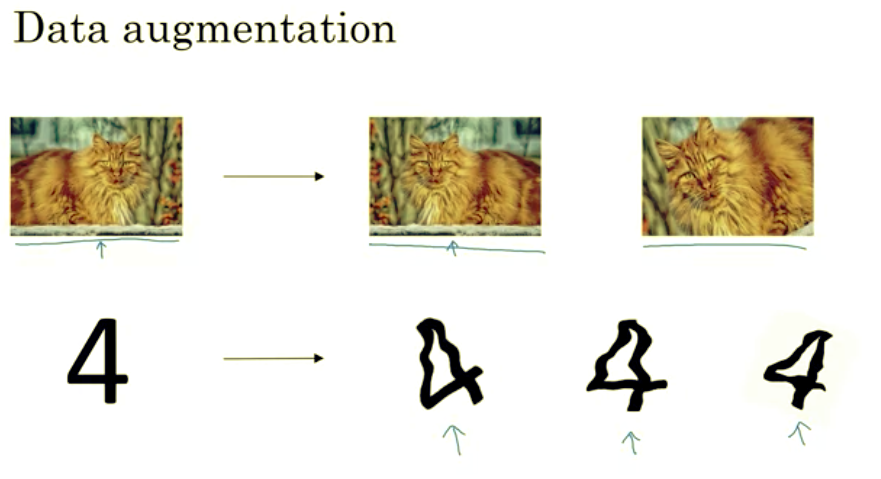
Early Stopping
There's one other technique that is often used called early stopping. So what you're going to do is as you run gradient descent you're going to plot your, either the training error, you'll use 01 classification error on the training set. Or just plot the cost function J optimizing, and that should decrease monotonically, like so, all right? Because as you trade, hopefully, you're trading around your cost function J should decrease.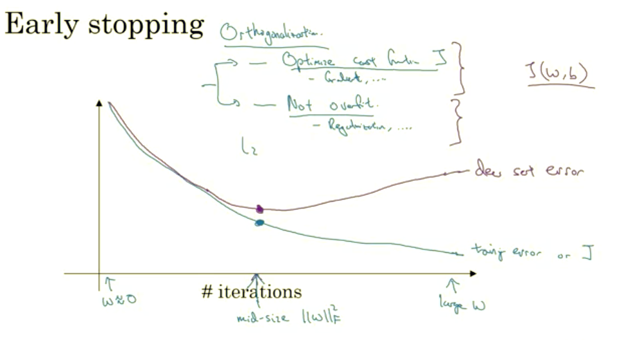
And so similar to L2 regularization by picking a neural network with smaller norm for your parameters w, hopefully your neural network is over fitting less. And the term early stopping refers to the fact that you’re just stopping the training of your neural network earlier.
Downside of early stopping
I sometimes use early stopping when training a neural network. But it does have one downside, let me explain. I think of the machine learning process as comprising several different steps. One, is that you want an algorithm to optimize the cost function j and we have various tools to do that, such as grade intersect. And then we'll talk later about other algorithms, like momentum and RMS prop and Atom and so on. But after optimizing the cost function j, you also wanted to not over-fit. And we have some tools to do that such as your regularization, getting more data and so on. Now in machine learning, we already have so many hyper-parameters it surge over. It's already very complicated to choose among the space of possible algorithms. And so I find machine learning easier to think about when you have one set of tools for optimizing the cost function J, and when you're focusing on authorizing the cost function J. All you care about is finding w and b, so that J(w,b) is as small as possible. You just don't think about anything else other than reducing this. And then it's completely separate task to not over fit, in other words, to reduce variance. And when you're doing that, you have a separate set of tools for doing it. And this principle is sometimes called orthogonalization. And there's this idea, that you want to be able to think about one task at a time. I'll say more about orthorganization in a later section, so if you don't fully get the concept yet, don't worry about it. But, to me the main downside of early stopping is that this couples these two tasks. So you no longer can work on these two problems independently, because by stopping gradient decent early, you're sort of breaking whatever you're doing to optimize cost function J, because now you're not doing a great job reducing the cost function J. You've sort of not done that that well. And then you also simultaneously trying to not over fit. So instead of using different tools to solve the two problems, you're using one that kind of mixes the two. And this just makes the set of things you could try are more complicated to think about. Rather than using early stopping, one alternative is just use L2 regularization then you can just train the neural network as long as possible. I find that this makes the search space of hyper parameters easier to decompose, and easier to search over. But the downside of this though is that you might have to try a lot of values of the regularization parameter lambda. And so this makes searching over many values of lambda more computationally expensive. And the advantage of early stopping is that running the gradient descent process just once, you get to try out values of small w, mid-size w, and large w, without needing to try a lot of values of the L2 regularization hyperparameter lambda.If this concept doesn’t completely make sense to you yet, don’t worry about it. We’re going to talk about it in greater detail in a later section, I think this will make a bit more sense. Despite it’s disadvantages, many people do use it. I personally prefer to just use L2 regularization and try different values of lambda. That’s assuming you can afford the computation to do so. But early stopping does let you get a similar effect without needing to explicitly try lots of different values of lambda. So you’ve now seen how to use data augmentation as well as if you wish early stopping in order to reduce variance or prevent over fitting your neural network. Next let’s talk about some techniques for setting up your optimization problem to make your training go quickly.