Naive Bayes Intution
What is Bayes Formulae
Implementation Naive Bayes with socail network database
Please Click Here to download the dataset used for this example

What is Naive Bayes

In machine learning, naïve Bayes classifiers are a family of simple "probabilistic classifiers" based on applying Bayes' theorem with strong (naïve) independence assumptions between the features. They are among the simplest Bayesian network models. But they could be coupled with Kernel density estimation and achieve higher accuracy levels.

The Naive Bayesian classifier is based on Bayes’ theorem with the independence assumptions between predictors. A Naive Bayesian model is easy to build, with no complicated iterative parameter estimation which makes it particularly useful for very large datasets. Despite its simplicity, the Naive Bayesian classifier often does surprisingly well and is widely used because it often outperforms more sophisticated classification methods.

Algorithm

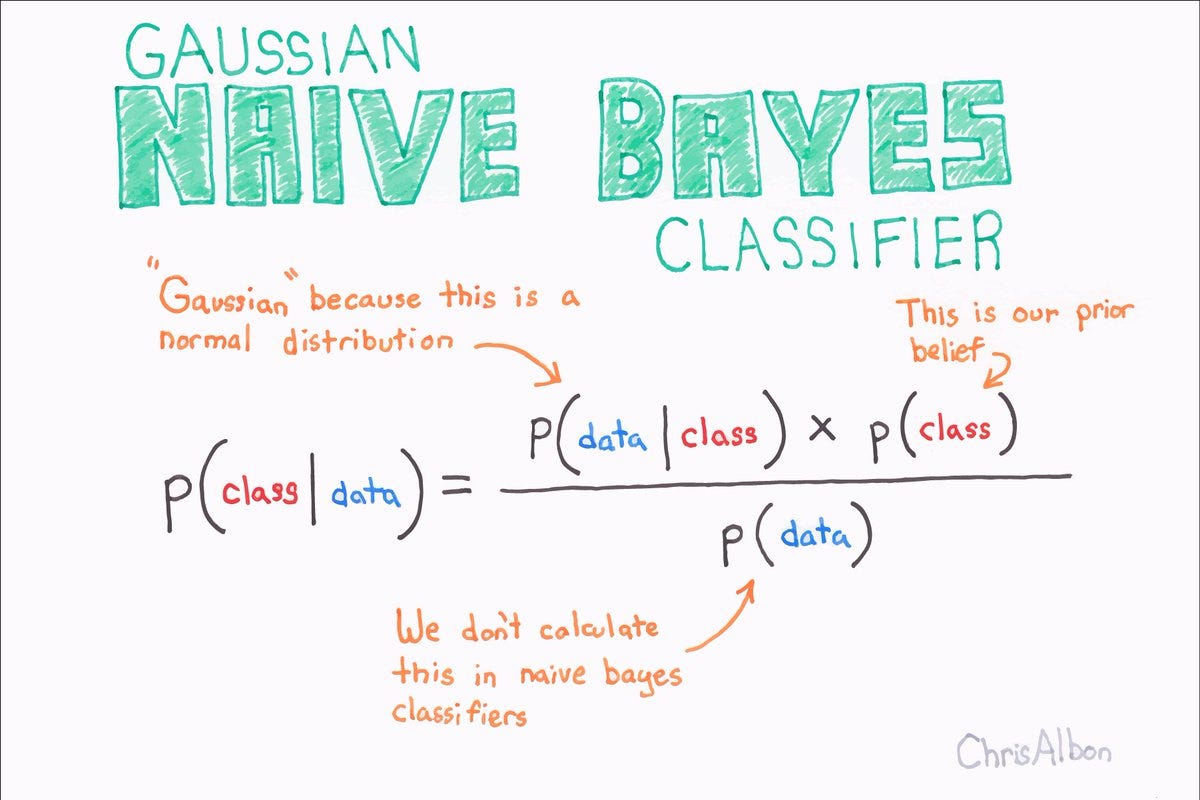
Bayes theorem provides a way of calculating the posterior probability, P(c|x), from P(c), P(x), and P(x|c). Naive Bayes classifier assume that the effect of the value of a predictor (x) on a given class (c) is independent of the values of other predictors. This assumption is called class conditional independence.

Bayes Formulae

This can also be interpreted as

Implementation of Naive Bayes Classifier

Import libraries

import pandas as pd
import numpy as np
from matplotlib import pyplot as plt

df = pd.read_csv('Social_Network_Ads.csv')
df.describe()

df.shape

(400, 5)

df.head(5)

# here purchased is our dependent variable

#Converting string values to int so that our model can fit to the dataset better
from sklearn.preprocessing import LabelEncoder
scall = LabelEncoder()
df.iloc[: , 1] = scall.fit_transform(df.iloc[:,1])
df.head(5)

# Splitting x and y here
x = df.iloc[: , 1:4].values
y = df.iloc[:, 4].values

print(x[:5])

[[    1    19 19000]
 [    1    35 20000]
 [    0    26 43000]
 [    0    27 57000]
 [    1    19 76000]]

# train test split
from sklearn.model_selection import train_test_split
x_train , x_test , y_train , y_test = train_test_split(x, y , train_size = 0.8, test_size = 0.2 , random_state = 1)
print(x_train.shape, x_test.shape , y_train.shape)

(320, 3) (80, 3) (320,)

Model fitting and predicting score

from sklearn.naive_bayes import GaussianNB
classifier = GaussianNB()
classifier.fit(x_train, y_train)

GaussianNB(priors=None, var_smoothing=1e-09)

#predicting values
y_pred = classifier.predict(x_test)

Evaluating model prediction

from sklearn.metrics import accuracy_score, confusion_matrix
print('accuracy oy model is : ', accuracy_score(y_test, y_pred))
print('Confusion Matrix:','\n', confusion_matrix(y_test, y_pred))

accuracy oy model is :  0.8625
Confusion Matrix: 
 [[41  7]
 [ 4 28]]

## we have 86% accuracy in our model

plt.scatter(x_test[:, 1],y_test,color ='red')
plt.scatter(x_test[:,1],y_pred, color = 'blue')
plt.show()

We can clearly see the results the graph The values that are in a different color are predicted wrong rest are right

	User ID	Age	EstimatedSalary	Purchased
count	4.000000e+02	400.000000	400.000000	400.000000
mean	1.569154e+07	37.655000	69742.500000	0.357500
std	7.165832e+04	10.482877	34096.960282	0.479864
min	1.556669e+07	18.000000	15000.000000	0.000000
25%	1.562676e+07	29.750000	43000.000000	0.000000
50%	1.569434e+07	37.000000	70000.000000	0.000000
75%	1.575036e+07	46.000000	88000.000000	1.000000
max	1.581524e+07	60.000000	150000.000000	1.000000

	User ID	Gender	Age	EstimatedSalary
0	15624510	Male	19	19000
1	15810944	Male	35	20000
2	15668575	Female	26	43000
3	15603246	Female	27	57000
4	15804002	Male	19	76000