Setting Up Optimisation

Note - These are my notes on DeepLearning Specialization Course for Setting Up Optimisation (Normalization | Vanishing/Exploding Gradients , Weight Initialization , Gradient Checking || Improving Deep Neural Networks

Introduction:
When training a neural network, one of the techniques that will speed up your training is if you normalize your inputs. Let’s see what that means. Let’s see if a training sets with two input features. So the input features x are two dimensional, and here’s a scatter plot of your training set.

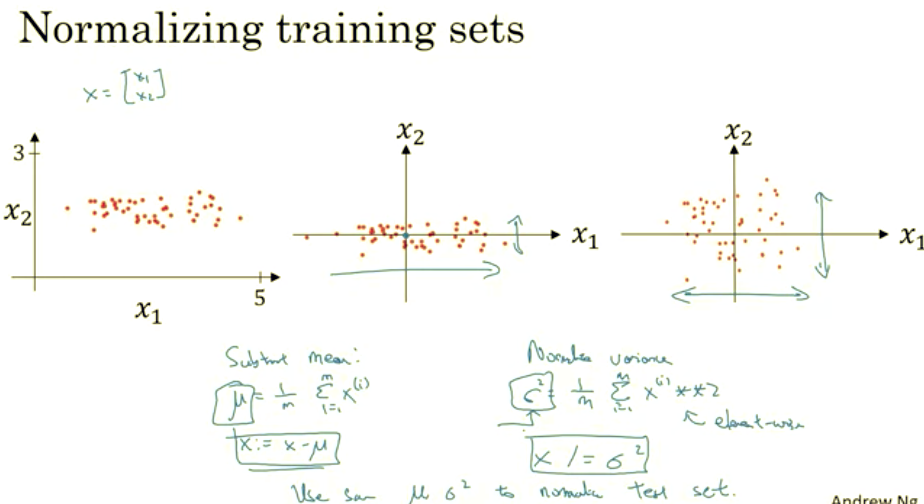
Normalizing your inputs corresponds to two steps. The first is to subtract out or to zero out the mean. So you set mu = 1 over M sum over I of Xi. So this is a vector, and then X gets set as X- mu for every training example, so this means you just move the training set until it has 0 mean. And then the second step is to normalize the variances. So notice here that the feature X1 has a much larger variance than the feature X2 here. So what we do is set sigma = 1 over m sum of Xipower2.

I guess this is a element y squaring. And so now sigma squared is a vector with the variances of each of the features, and notice we’ve already subtracted out the mean, so Xi squared, element y squared is just the variances. And you take each example and divide it by this vector sigma squared. And so in pictures, you end up with this. Where now the variance of X1 and X2 are both equal to one.
And one tip, if you use this to scale your training data, then use the same mu and sigma squared to normalize your test set, right? In particular, you don’t want to normalize the training set and the test set differently. Whatever this value is and whatever this value is, use them in these two formulas so that you scale your test set in exactly the same way, rather than estimating mu and sigma squared separately on your training set and test set. Because you want your data, both training and test examples, to go through the same transformation defined by the same mu and sigma squared calculated on your training data.
So, why do we do Normalization?

Why do we want to normalize the input features? Recall that a cost function is defined as written on the top right. It turns out that if you use unnormalized input features, it’s more likely that your cost function will look like this, it’s a very squished out bowl, very elongated cost function, where the minimum you’re trying to find is maybe over there. But if your features are on very different scales, say the feature X1 ranges from 1 to 1,000, and the feature X2 ranges from 0 to 1, then it turns out that the ratio or the range of values for the parameters w1 and w2 will end up taking on very different values. And so maybe these axes should be w1 and w2, but I’ll plot w and b, then your cost function can be a very elongated bowl like that.

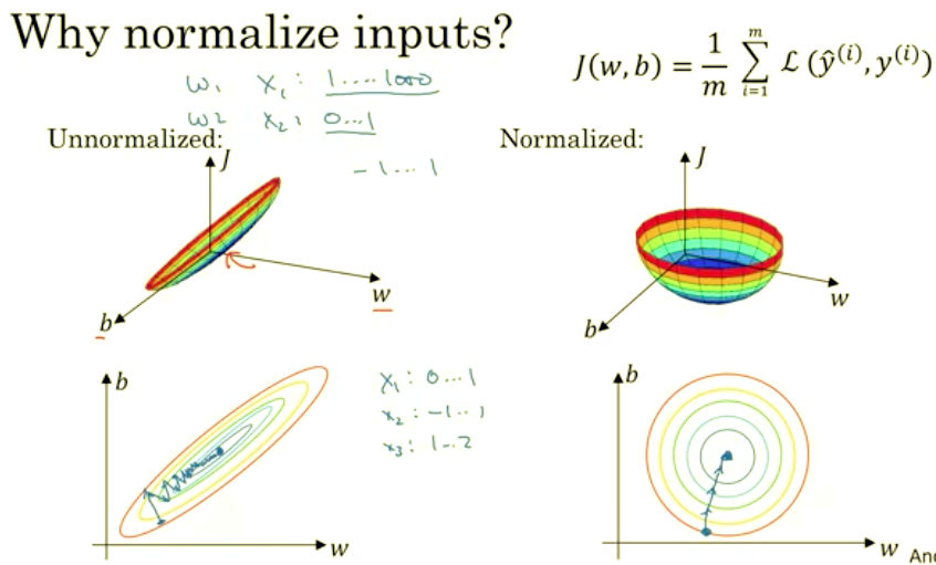
So if you part the contours of this function, you can have a very elongated function like that. Whereas if you normalize the features, then your cost function will on average look more symmetric. And if you’re running gradient descent on the cost function like the one on the left, then you might have to use a very small learning rate because if you’re here that gradient descent might need a lot of steps to oscillate back and forth before it finally finds its way to the minimum. Whereas if you have a more spherical contours, then wherever you start gradient descent can pretty much go straight to the minimum. You can take much larger steps with gradient descent rather than needing to oscillate around like like the picture on the left. Of course in practice w is a high-dimensional vector, and so trying to plot this in 2D doesn’t convey all the intuitions correctly. But the rough intuition that your cost function will be more round and easier to optimize when your features are all on similar scales. Not from one to 1000, zero to one, but mostly from minus one to one or of about similar variances of each other. That just makes your cost function J easier and faster to optimize. In practice if one feature, say X1, ranges from zero to one, and X2 ranges from minus one to one, and X3 ranges from one to two, these are fairly similar ranges, so this will work just fine. It’s when they’re on dramatically different ranges like ones from 1 to a 1000, and the another from 0 to 1, that that really hurts your authorization algorithm. But by just setting all of them to a 0 mean and say, variance 1, like we did in the last slide, that just guarantees that all your features on a similar scale and will usually help your learning algorithm run faster. So, if your input features came from very different scales, maybe some features are from 0 to 1, some from 1 to 1,000, then it’s important to normalize your features. If your features came in on similar scales, then this step is less important. Although performing this type of normalization pretty much never does any harm, so I’ll often do it anyway if I’m not sure whether or not it will help with speeding up training for your algebra.
So that’s it for normalizing your input features. Next, let’s keep talking about ways to speed up the training of your new network.
When training a neural network, one of the techniques
Vanishing / Exploding gradients
One of the problems of training neural network, especially very deep neural networks, is data vanishing and exploding gradients. What that means is that when you’re training a very deep network your derivatives or your slopes can sometimes get either very, very big or very, very small, maybe even exponentially small, and this makes training difficult. In this Topic you see what this problem of exploding and vanishing gradients really means, as well as how you can use careful choices of the random weight initialization to significantly reduce this problem. Unless you’re training a very deep neural network like this, to save space on the slide, I’ve drawn it as if you have only two hidden units per layer, but it could be more as well. But this neural network will have parameters W1, W2, W3 and so on up to WL.

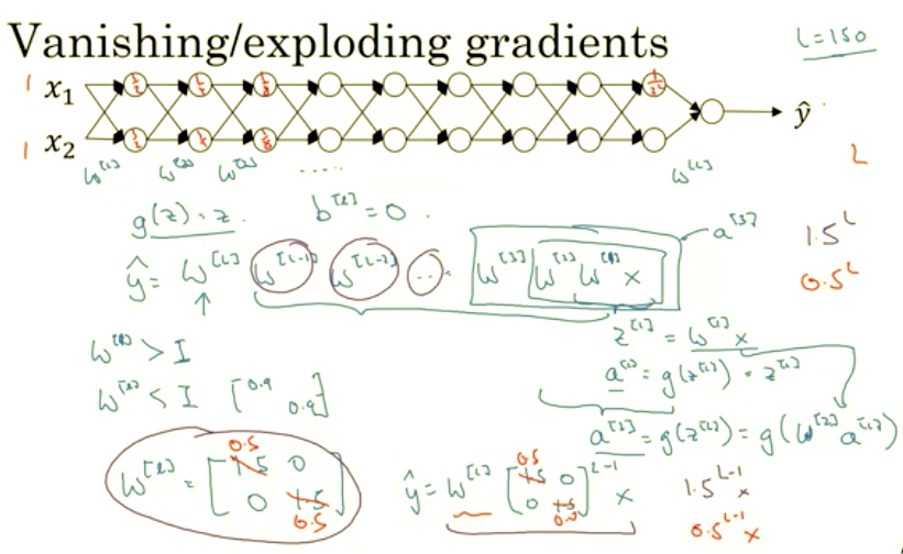
For the sake of simplicity, let’s say we’re using an activation function G of Z equals Z, so linear activation function. And let’s ignore B, let’s say B of L equals zero. So in that case you can show that the output Y will be WL times WL minus one times WL minus two, dot, dot, dot down to the W3, W2, W1 times X. But if you want to just check my math, W1 times X is going to be Z1, because B is equal to zero. So Z1 is equal to, I guess, W1 times X and then plus B which is zero. But then A1 is equal to G of Z1.
But because we use linear activation function, this is just equal to Z1. So this first term W1X is equal to A1. And then by the reasoning you can figure out that W2 times W1 times X is equal to A2, because that’s going to be G of Z2, is going to be G of W2 times A1 which you can plug that in here. So this thing is going to be equal to A2, and then this thing is going to be A3 and so on until the protocol of all these matrices gives you Y-hat, not Y. Now, let’s say that each of you weight matrices WL is just a little bit larger than one times the identity. So it’s 1.5_1.5_0_0.
Technically, the last one has different dimensions so maybe this is just the rest of these weight matrices. Then Y-hat will be, ignoring this last one with different dimension, this 1.5_0_0_1.5 matrix to the power of L minus 1 times X, because we assume that each one of these matrices is equal to this thing. It’s really 1.5 times the identity matrix, then you end up with this calculation. And so Y-hat will be essentially 1.5 to the power of L, to the power of L minus 1 times X, and if L was large for very deep neural network, Y-hat will be very large. In fact, it just grows exponentially, it grows like 1.5 to the number of layers. And so if you have a very deep neural network, the value of Y will explode. Now, conversely, if we replace this with 0.5, so something less than 1, then this becomes 0.5 to the power of L. This matrix becomes 0.5 to the L minus one times X, again ignoring WL. And so each of your matrices are less than 1, then let’s say X1, X2 were one one, then the activations will be one half, one half, one fourth, one fourth, one eighth, one eighth, and so on until this becomes one over two to the L. So the activation values will decrease exponentially as a function of the def, as a function of the number of layers L of the network. So in the very deep network, the activations end up decreasing exponentially.

So the intuition I hope you can take away from this is that at the weights W, if they’re all just a little bit bigger than one or just a little bit bigger than the identity matrix, then with a very deep network the activations can explode. And if W is just a little bit less than identity. So this maybe here’s 0.9, 0.9, then you have a very deep network, the activations will decrease exponentially. And even though I went through this argument in terms of activations increasing or decreasing exponentially as a function of L, a similar argument can be used to show that the derivatives or the gradients the computer is going to send will also increase exponentially or decrease exponentially as a function of the number of layers. With some of the modern neural networks, L equals 150.
Microsoft recently got great results with 152 layer neural network. But with such a deep neural network, if your activations or gradients increase or decrease exponentially as a function of L, then these values could get really big or really small. And this makes training difficult, especially if your gradients are exponentially smaller than L, then gradient descent will take tiny little steps. It will take a long time for gradient descent to learn anything. To summarize, you’ve seen how deep networks suffer from the problems of vanishing or exploding gradients. In fact, for a long time this problem was a huge barrier to training deep neural networks.
It turns out there’s a partial solution that doesn’t completely solve this problem but it helps a lot which is careful choice of how you initialize the weights. To see that, let’s go to the next Topic.
One of the problems of training neural network, especially very deep neural networks, is data vanishing. What that means is that when you’re training a very deep network your derivatives or your slopes can sometimes get either very, very big or very, very small, maybe even exponentially small, and this makes training difficult. In this Topic you see what this problem of exploding and vanishing gradients really means, as well as how you can use careful choices of the random weight initialization to significantly reduce this problem. Unless you’re training a very deep neural network like this, to save space on the slide, I’ve drawn it as if you have only two hidden units per layer, but it could be more as well. But this neural network will have parameters W1, W2, W3 and so on up to WL.

Technically, the last one has different dimensions so maybe this is just the rest of these weight matrices. Then Y-hat will be, ignoring this last one with different dimension, this 1.5_0_0_1.5 matrix to the power of L minus 1 times X, because we assume that each one of these matrices is equal to this thing. It’s really 1.5 times the identity matrix, then you end up with this calculation. And so Y-hat will be essentially 1.5 to the power of L, to the power of L minus 1 times X, and if L was large for very deep neural network, Y-hat will be very large. In fact, it just grows exponentially, it grows like 1.5 to the number of layers. And so if you have a very deep neural network, the value of Y will explode. Now, conversely, if we replace this with 0.5, so something less than 1, then this becomes 0.5 to the power of L. This matrix becomes 0.5 to the L minus one times X, again ignoring WL. And so each of your matrices are less than 1, then let’s say X1, X2 were one one, then the activations will be one half, one half, one fourth, one fourth, one eighth, one eighth, and so on until this becomes one over two to the L. So the activation values will decrease exponentially as a function of the def, as a function of the number of layers L of the network. So in the very deep network, the activations end up decreasing exponentially.

So the intuition I hope you can take away from this is that at the weights W, if they're all just a little bit bigger than one or just a little bit bigger than the identity matrix, then with a very deep network the activations can explode. And if W is just a little bit less than identity. So this maybe here's 0.9, 0.9, then you have a very deep network, the activations will decrease exponentially. And even though I went through this argument in terms of activations increasing or decreasing exponentially as a function of L, a similar argument can be used to show that the derivatives or the gradients the computer is going to send will also increase exponentially or decrease exponentially as a function of the number of layers. With some of the modern neural networks, L equals 150. Microsoft recently got great results with 152 layer neural network. But with such a deep neural network, if your activations or gradients increase or decrease exponentially as a function of L, then these values could get really big or really small. And this makes training difficult, especially if your gradients are exponentially smaller than L, then gradient descent will take tiny little steps. It will take a long time for gradient descent to learn anything. To summarize, you've seen how deep networks suffer from the problems of vanishing or exploding gradients. In fact, for a long time this problem was a huge barrier to training deep neural networks. It turns out there's a partial solution that doesn't completely solve this problem but it helps a lot which is careful choice of how you initialize the weights. To see that, let's go to the next Topic. One of the problems of training neural network, especially very deep neural networks, is data vanishing

_3>Weight Initialization for Deep Networks_3>
In the last paragraph you saw how very deep neural networks can have the problems of vanishing and exploding gradients. It turns out that a partial solution to this, doesn’t solve it entirely but helps a lot, is better or more careful choice of the random initialization for your neural network.
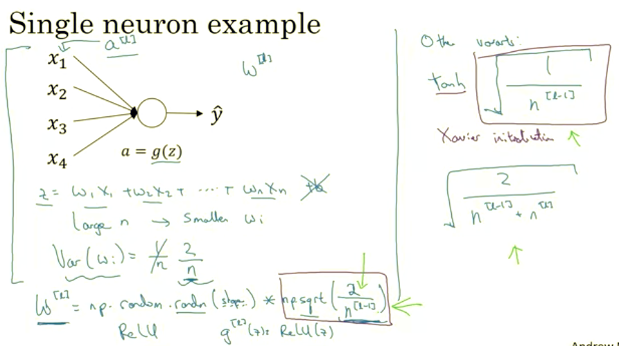
_4>Single Neuron_4>
To understand this, let’s start with the example of initializing the ways for a single neuron, and then we’re go on to generalize this to a deep network. Let’s go through this with an example with just a single neuron, and then we’ll talk about the deep net later. So with a single neuron, you might input four features, x1 through x4, and then you have some a=g(z) and then it outputs some y. And later on for a deeper net, you know these inputs will be right, some layer a(l), but for now let’s just call this x for now.

So z is going to be equal to w1x1 + w2x2 +... + I guess WnXn. And let's set b=0 so, you know, let's just ignore b for now. So in order to make z not blow up and not become too small, you notice that the larger n is, the smaller you want Wi to be, right? Because z is the sum of the WiXi. And so if you're adding up a lot of these terms, you want each of these terms to be smaller. One reasonable thing to do would be to set the variance of Wi to be equal to 1 over n, where n is the number of input features that's going into a neuron. So in practice, what you can do is set the weight matrix W for a certain layer to be np.random.randn you know, and then whatever the shape of the matrix is for this out here, and then times square root of 1 over the number of features that I fed into each neuron in layer l. So there's going to be n(l-1) because that's the number of units that I'm feeding into each of the units in layer l. _4>Using RElu Activation Function:_4> It turns out that if you're using a ReLu activation function that, rather than 1 over n it turns out that, set in the variance of 2 over n works a little bit better. So you often see that in initialization, especially if you're using a ReLu activation function. So if gl(z) is ReLu(z), oh and it depends on how familiar you are with random variables. It turns out that something, a Gaussian random variable and then multiplying it by a square root of this, that sets the variance to be quoted this way, to be 2 over n. And the reason I went from n to this n superscript l-1 was, in this example with logistic regression which is at n input features, but the more general case layer l would have n(l-1) inputs each of the units in that layer. So if the input features of activations are roughly mean 0 and standard variance and variance 1 then this would cause z to also take on a similar scale. And this doesn't solve, but it definitely helps reduce the vanishing, exploding gradients problem, because it's trying to set each of the weight matrices w, you know, so that it's not too much bigger than 1 and not too much less than 1 so it doesn't explode or vanish too quickly. I've just mention some other variants. The version we just described is assuming a ReLu activation function and this by a paper by [inaudible]. _4>Using TanH Activation Function: _4> A few other variants, if you are using a TanH activation function then there's a paper that shows that instead of using the constant 2, it's better use the constant 1 and so 1 over this instead of 2. And so you multiply it by the square root of this. So this square root term will replace this term and you use this if you're using a TanH activation function. This is called Xavier initialization. And another version we're taught by Yoshua Bengio and his colleagues, you might see in some papers, but is to use this formula, which you know has some other theoretical justification, but I would say if you're using a ReLu activation function, which is really the most common activation function, I would use this formula. If you're using TanH you could try this version instead, and some authors will also use this. But in practice I think all of these formulas just give you a starting point. It gives you a default value to use for the variance of the initialization of your weight matrices. If you wish the variance here, this variance parameter could be another thing that you could tune with your hyperparameters. So you could have another parameter that multiplies into this formula and tune that multiplier as part of your hyperparameter surge. Sometimes tuning the hyperparameter has a modest size effect.

It's not one of the first hyperparameters I would usually try to tune, but I've also seen some problems where tuning this helps a reasonable amount. But this is usually lower down for me in terms of how important it is relative to the other hyperparameters you can tune. So I hope that gives you some intuition about the problem of vanishing or exploding gradients as well as choosing a reasonable scaling for how you initialize the weights. Hopefully that makes your weights not explode too quickly and not decay to zero too quickly, so you can train a reasonably deep network without the weights or the gradients exploding or vanishing too much. When you train deep networks, this is another trick that will help you make your neural networks trained much more quickly.

_4>Numerical approximation of gradients_4>
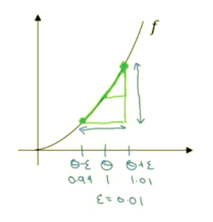
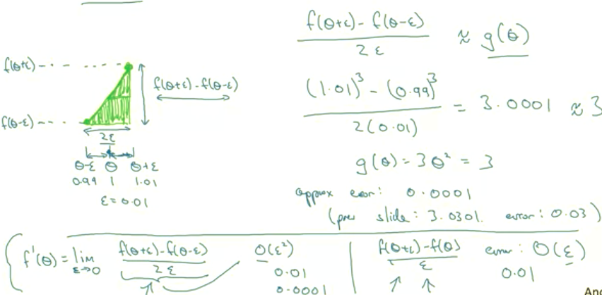
When you implement back propagation you’ll find that there’s a test called creating checking that can really help you make sure that your implementation of back prop is correct. Because sometimes you write all these equations and you’re just not 100% sure if you’ve got all the details right and internal back propagation. So in order to build up to gradient and checking, let’s first talk about how to numerically approximate computations of gradients and in the next Topic, we’ll talk about how you can implement gradient checking to make sure the implementation of backdrop is correct. So lets take the function f and replot it here and remember this is f of theta equals theta cubed, and let’s again start off to some value of theta. Let’s say theta equals 1. Now instead of just nudging theta to the right to get theta plus epsilon, we’re going to nudge it to the right and nudge it to the left to get theta minus epsilon, as was theta plus epsilon. So this is 1, this is 1.01, this is 0.99 where, again, epsilon is same as before, it is 0.01.
It turns out that rather than taking this little triangle and computing the height over the width, you can get a much better estimate of the gradient if you take this point, f of theta minus epsilon and this point, and you instead compute the height over width of this bigger triangle. So for technical reasons which I won’t go into, the height over width of this bigger green triangle gives you a much better approximation to the derivative at theta. And you saw it yourself, taking just this lower triangle in the upper right is as if you have two triangles, right? This one on the upper right and this one on the lower left. And you’re kind of taking both of them into account by using this bigger green triangle. So rather than a one sided difference, you’re taking a two sided difference.

So let's work out the math. This point here is F of theta plus epsilon. This point here is F of theta minus epsilon. So the height of this big green triangle is f of theta plus epsilon minus f of theta minus epsilon. And then the width, this is 1 epsilon, this is 2 epsilon. So the width of this green triangle is 2 epsilon. So the height of the width is going to be first the height, so that's F of theta plus epsilon minus F of theta minus epsilon divided by the width. So that was 2 epsilon which we write that down here. And this should hopefully be close to g of theta. So plug in the values, remember f of theta is theta cubed. So theta plus epsilon is 1.01. So I take a cube of that minus 0.99 theta cube of that divided by 2 times 0.01. Feel free to practice in the calculator. You should get that this is 3.0001.

So this two sided difference way of approximating the derivative you find that this is extremely close to 3. And so this gives you a much greater confidence that g of theta is probably a correct implementation of the derivative of F. _4>Single Sided Difference:_4> When you use this method for grading, checking and back propagation, this turns out to run twice as slow as you were to use a one-sided defferense. It turns out that in practice I think it's worth it to use this other method because it's just much more accurate. The little bit of optional theory for those of you that are a little bit more familiar of Calculus, it turns out that, and it's okay if you don't get what I'm about to say here. But it turns out that the formal definition of a derivative is for very small values of epsilon is f of theta plus epsilon minus f of theta minus epsilon over 2 epsilon. And the formal definition of derivative is in the limits of exactly that formula on the right as epsilon those as 0. And the definition of unlimited is something that you learned if you took a Calculus class but I won't go into that here. And it turns out that for a non zero value of epsilon, you can show that the error of this approximation is on the order of epsilon squared, and remember epsilon is a very small number. So if epsilon is 0.01 which it is here then epsilon squared is 0.0001. The big O notation means the error is actually some constant times this, but this is actually exactly our approximation error. So the big O constant happens to be 1. Whereas in contrast if we were to use this formula, the other one, then the error is on the order of epsilon. And again, when epsilon is a number less than 1, then epsilon is actually much bigger than epsilon squared which is why this formula here is actually much less accurate approximation than this formula on the left. Which is why when doing gradient checking, we rather use this two-sided difference when you compute f of theta plus epsilon minus f of theta minus epsilon and then divide by 2 epsilon rather than just one sided difference which is less accurate. <

If you didn't understand my last two comments, all of these things are on here. Don't worry about it. That's really more for those of you that are a bit more familiar with Calculus, and with numerical approximations. _4>TakeAway:_4> But the takeaway is that this two-sided difference formula is much more accurate. And so that's what we're going to use when we do gradient checking in the next Topic. So you've seen how by taking a two sided difference, you can numerically verify whether or not a function g, g of theta that someone else gives you is a correct implementation of the derivative of a function f. Let's now see how we can use this to verify whether or not your back propagation implementation is correct or if there might be a bug in there that you need to go and tease out

Credits to the teacher