Random Forest Classification

• Random Forest Intution
• Why Random Forest
• Implementation Random Forest with social network database
• Please Click Here to download the dataset used for this example

What is Random Forest ?

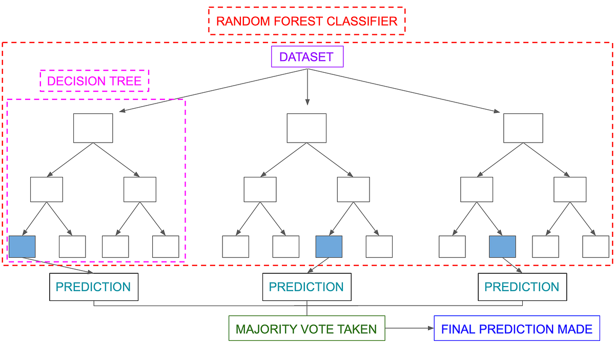
Random Forest is an ensemble method that combines multiple decision trees to classify, So the result of random forest is usually better than decision trees
Random forests is a supervised learning algorithm. It can be used both for classification and regression. It is also the most flexible and easy to use algorithm. A forest is comprised of trees. It is said that the more trees it has, the more robust a forest is. Random forests creates decision trees on randomly selected data samples, gets prediction from each tree and selects the best solution by means of voting. It also provides a pretty good indicator of the feature importance.

Random forests has a variety of applications, such as recommendation engines, image classification and feature selection. It can be used to classify loyal loan applicants, identify fraudulent activity and predict diseases. It lies at the base of the Boruta algorithm, which selects important features in a dataset.

Implementation of Random Forest Classifier

Import libraries

In [1]:

import pandas as pd
import numpy as np
from matplotlib import pyplot as plt

In [2]:

df = pd.read_csv('Social_Network_Ads.csv')
df.describe()

Out[2]:

	User ID	Age	EstimatedSalary	Purchased
count	4.000000e+02	400.000000	400.000000	400.000000
mean	1.569154e+07	37.655000	69742.500000	0.357500
std	7.165832e+04	10.482877	34096.960282	0.479864
min	1.556669e+07	18.000000	15000.000000	0.000000
25%	1.562676e+07	29.750000	43000.000000	0.000000
50%	1.569434e+07	37.000000	70000.000000	0.000000
75%	1.575036e+07	46.000000	88000.000000	1.000000
max	1.581524e+07	60.000000	150000.000000	1.000000

In [3]:

df.shape

Out[3]:

(400, 5)

In [4]:

df.head(5)

Out[4]:

	User ID	Gender	Age	EstimatedSalary	Purchased
0	15624510	Male	19	19000	0
1	15810944	Male	35	20000	0
2	15668575	Female	26	43000	0
3	15603246	Female	27	57000	0
4	15804002	Male	19	76000	0

In [5]:

# here purchased is our dependent variable

In [6]:

#Converting string values to int so that our model can fit to the dataset better
from sklearn.preprocessing import LabelEncoder
scall = LabelEncoder()
df.iloc[: , 1] = scall.fit_transform(df.iloc[:,1])
df.head(5)

Out[6]:

	User ID	Gender	Age	EstimatedSalary	Purchased
0	15624510	1	19	19000	0
1	15810944	1	35	20000	0
2	15668575	0	26	43000	0
3	15603246	0	27	57000	0
4	15804002	1	19	76000	0

In [7]:

# Splitting x and y here
x = df.iloc[: , 1:4].values
y = df.iloc[:, 4].values

print(x[:5])

[[    1    19 19000]
 [    1    35 20000]
 [    0    26 43000]
 [    0    27 57000]
 [    1    19 76000]]

In [8]:

# train test split
from sklearn.model_selection import train_test_split
x_train , x_test , y_train , y_test = train_test_split(x, y , train_size = 0.8, test_size = 0.2 , random_state = 1)
print(x_train.shape, x_test.shape , y_train.shape)

(320, 3) (80, 3) (320,)

Model fitting and predicting score

In [9]:

from sklearn.ensemble import RandomForestClassifier
classifier = RandomForestClassifier()
classifier.fit(x_train, y_train)

/home/jupyterlab/conda/envs/python/lib/python3.6/site-packages/sklearn/ensemble/forest.py:246: FutureWarning: The default value of n_estimators will change from 10 in version 0.20 to 100 in 0.22.
  "10 in version 0.20 to 100 in 0.22.", FutureWarning)

Out[9]:

RandomForestClassifier(bootstrap=True, class_weight=None, criterion='gini',
            max_depth=None, max_features='auto', max_leaf_nodes=None,
            min_impurity_decrease=0.0, min_impurity_split=None,
            min_samples_leaf=1, min_samples_split=2,
            min_weight_fraction_leaf=0.0, n_estimators=10, n_jobs=None,
            oob_score=False, random_state=None, verbose=0,
            warm_start=False)

In [10]:

#predicting values
y_pred = classifier.predict(x_test)

Evaluating model prediction

In [11]:

from sklearn.metrics import accuracy_score, confusion_matrix
print('accuracy oy model is : ', accuracy_score(y_test, y_pred))
print('Confusion Matrix:','\n', confusion_matrix(y_test, y_pred))

accuracy oy model is :  0.8625
Confusion Matrix: 
 [[40  8]
 [ 3 29]]

In [12]:

## we have 86% accuracy in our model

## Out of all predictions 7+4 = 11 are incorrect prediction

In [13]:

plt.scatter(x_test[:, 1],y_test,color ='red')
plt.scatter(x_test[:,1],y_pred, color = 'blue')
plt.show()

We can clearly see the results the graph The values that are in a different color are predicted wrong rest are right