In this notebook we will compare all the regression model on a dataset with 10000 values.
Models we will cover and execute a working model for:
- Multiple Linear regression
- Polynomial Regression
- RBF kernel SVR
- Decision Trees
- Random Forest
You can download the data we used in this blog by - Clicking here
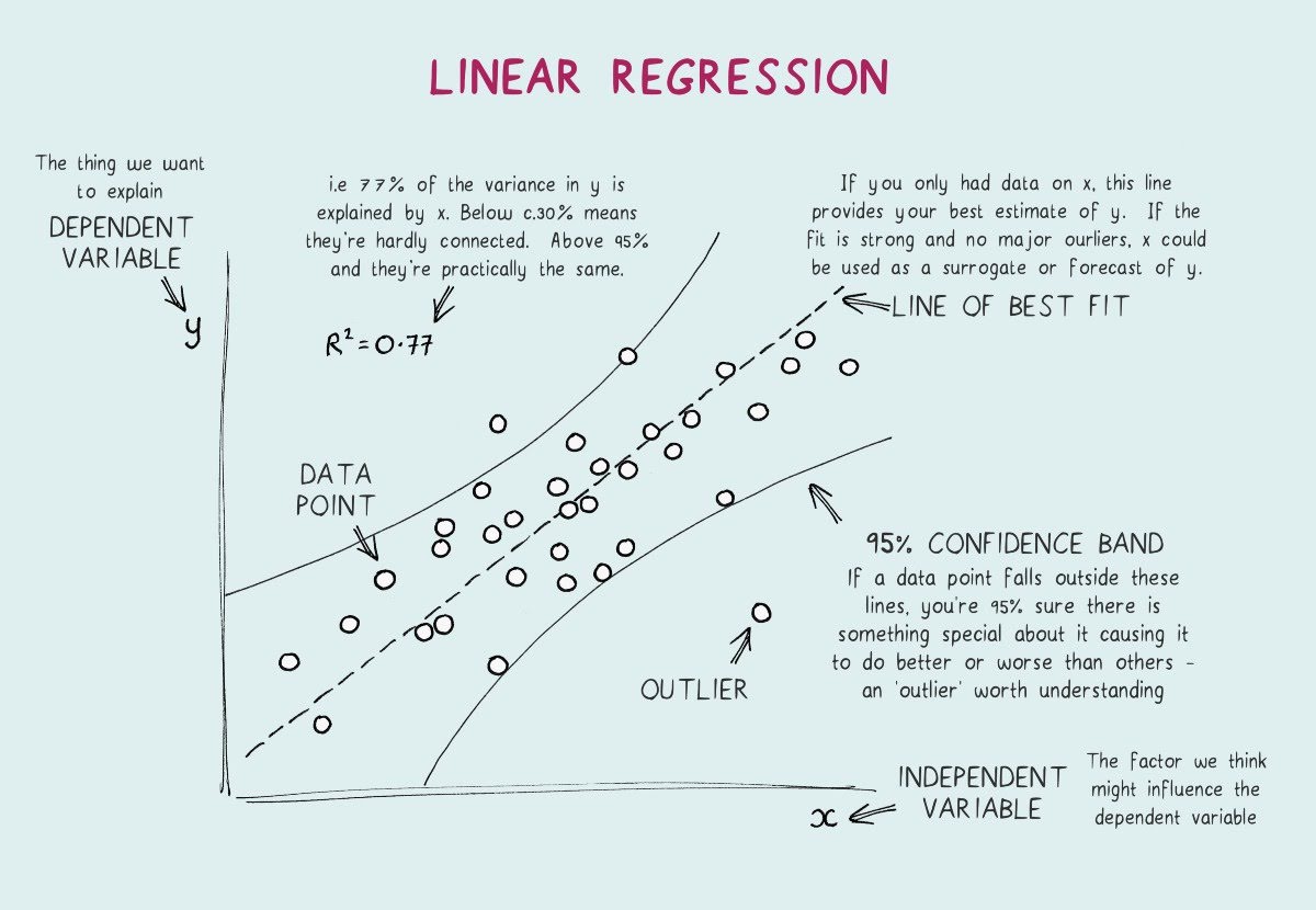
Here is an entensive example of a liner regression model for refresh of your memory :)
import pandas as pd
import numpy as np
from matplotlib import pyplot as plt
df = pd.read_excel('00.xlsx')
df.shape #10000 rows and 5 columns
df.head()
df.describe()
x = df.iloc[: , 0:4].values #.values will create an array instead of a dataframe object
y = df.iloc[: , 4:5].values
y.T
x.T
from sklearn.model_selection import train_test_split
#80-20 split
x_train, x_test , y_train, y_test = train_test_split(x, y, train_size = 0.8, random_state = 0)
x_train.shape
x_test.shape

plt.scatter(x[:, 0],y)

#doing covariance test
import statsmodels.api as sm
ols = sm.add_constant(x)
results = sm.OLS(y,x).fit()
print(results.summary())
from sklearn.linear_model import LinearRegression
regressor = LinearRegression()
regressor.fit(x_train , y_train)

#print intercept and coefficient
print(regressor.coef_, '\n', regressor.intercept_)
#visualizing results
plt.figure(figsize = (10,5))
plt.scatter(x[:,0] , y )
plt.plot(x_test[:,0], regressor.predict(x_test), color = 'red')
plt.xlabel('Independent Variable')
plt.ylabel('Dependent Variable')
plt.title('Multiple Linear Regression')
plt.show()

from sklearn.metrics import r2_score
r2_score(y_test,regressor.predict(x_test))
#closer the r2 to 1, better is the score
# importing libraries for polynomial transform
from sklearn.preprocessing import PolynomialFeatures
# for creating pipeline
from sklearn.pipeline import Pipeline
results = [('polynomial', PolynomialFeatures(degree = 5)) , ('model', LinearRegression())]
# creating pipeline and fitting it on data
pipe = Pipeline(results)
pipe.fit(x_train,y_train)
plt.scatter(x[:, 0],y, color = 'black')
plt.plot(x_test[:, 0], pipe.predict(x_test), color = 'purple')
plt.xlabel('Independent Variable')
plt.ylabel('Dependent Variable')
plt.title('Polynomial Regresion')
plt.show()

from sklearn.metrics import r2_score
r2_score(y_test, pipe.predict(x_test))

#this score is better than multiple linear regression
from sklearn.preprocessing import StandardScaler
sc_X = StandardScaler()
sc_y = StandardScaler()
X_train = sc_X.fit_transform(x_train)
Y_train = sc_y.fit_transform(y_train)


from sklearn.svm import SVR
regressor = SVR(kernel = 'rbf')
regressor.fit(X_train, Y_train)

y_pred = sc_y.inverse_transform(regressor.predict(sc_X.transform(x_test)))
np.set_printoptions(precision=2)
print(np.concatenate((y_pred.reshape(len(y_pred),1), y_test.reshape(len(y_test),1)),1))
plt.scatter(x[:, 0],y, color = 'black')
plt.plot(x_test[:, 0], y_pred, color = 'blue')
plt.xlabel('Independent Variable')
plt.ylabel('Dependent Variable')
plt.title('Support Vector Regresion')
plt.show()

from sklearn.metrics import r2_score
r2_score(y_test, y_pred)

#so far the best model is SVR
from sklearn.tree import DecisionTreeRegressor
treo = DecisionTreeRegressor(random_state = 0)

treo.fit(x_train , y_train)


#plotting the result after fitting
plt.scatter(x[:,0],y, color = 'purple')
plt.plot(x_test[:,0], treo.predict(x_test), color ='black')
plt.xlabel('Independent Variable')
plt.ylabel('Dependent Variable')
plt.title('Decision Tree Regression')
plt.show()

from sklearn.metrics import r2_score
r2_score(y_test, treo.predict(x_test))

#so far decision tree regression is the worst model
from sklearn.ensemble import RandomForestRegressor
rf = RandomForestRegressor(n_estimators = 200, random_state = 0)
rf.fit(x_train, y_train)


#plotting the result after fitting
plt.scatter(x[:,0],y, color = 'black')
plt.plot(x_test[:,0], rf.predict(x_test), color ='green')
plt.xlabel('Independent Variable')
plt.ylabel('Dependent Variable')
plt.title('Random Forest Regression')
plt.show()

from sklearn.metrics import r2_score
r2_score(y_test, rf.predict(x_test))

# Best results we have
Conclusion
Therefore the Random Forest Model Fits to our data well,
Considering the present scanario we will choose the random forest method for our further process
NOTE: To be considered that we have not taken to account overfitting and high variance low bais issue in this model.
Also we have not considered the hyperparameter tuning for any of the hperparameters involved.
More Content
If you want to see the separate implementation and theory of these models on the website with a different dataset.
Please click on these links below
- Simple Linear Regression - https://massivefile.com/simple_linear_regression/
- Multiple Linear regression - https://massivefile.com/multiple_linear_regression/
- Polynomial Regression - https://massivefile.com/PolynomialRegression/
- Non Linear Regerssion - https://massivefile.com/NoneLinearRegression/
- RBF kernel SVR - https://massivefile.com/supportvectorregression/
- Decision Trees - https://massivefile.com/decisiontreeregression/
- Random Forest - https://massivefile.com/randomforestregression/
Learn About Data Preprocessing : Click Here